Summary
On 7th November 1940 (four months after its opening), the Tacoma Narrows Bridge collapsed when the wind speed was 19 m/s, far below its specified load capacities. The collapse was associated with aerodynamic, not structural forces. A thin, solid-sided deck was so twisted against the wind that the hangers could no longer hold. Currently, that collapse can be replicated by modern wind-tunnel testing and finite element modeling, but the cause of it remains controversial. This case study examines the failure, reveals what recent research has made clear, and makes lessons concerning testing, deck shape, vibration control and design codes that are still applicable to the current longest bridges.
Key Words: Aerodynamics, wind-tunnel testing, Tacoma Narrows Bridge, width-depth ratio
Background
The Tacoma Narrows Bridge was opened on 1st July 1940 and connected Tacoma, Washington, and the Kitsap Peninsula. At the time, it was the third-longest suspension bridge in the world and the main span of the bridge measured 2,800 feet (850 m). Its architects sought austerity and style. They not only had solid plate girders with plates 8 feet deep, but also a deck, only 39 feet wide, giving a width-depth ratio of 5:1 that formed an H-shaped cross-section, perfected to act like a bluff body but not a streamlined body.1 The design was also cost-driven. A more substantial stiffening truss was pondered over, but a less expensive, thinner plate-girder design was used, and the slimness of the bridge was proclaimed an advance, instead of being challenged.
- Tacoma Narrows, first bridge, 1940: main span 2,800 feet; 39 feet between the cables; stiffening girder or truss 8 feet deep, 1 in 350 of the span; width to depth 4.9 to 1. The bridge the case study is about.
- Bronx-Whitestone, 1939: main span 2,300 feet; 74 feet between the cables; stiffening girder or truss 11 feet deep, 1 in 209 of the span; width to depth 6.7 to 1.
- Golden Gate, 1937: main span 4,200 feet; 90 feet between the cables; stiffening girder or truss 25 feet deep, 1 in 168 of the span; width to depth 3.6 to 1.
- Tacoma Narrows, second bridge, 1950: main span 2,800 feet; 60 feet between the cables; stiffening girder or truss 33 feet deep, 1 in 85 of the span; width to depth 1.8 to 1.
- San Francisco–Oakland Bay, 1936: main span 2,310 feet; 66 feet between the cables; stiffening girder or truss 30 feet deep, 1 in 77 of the span; width to depth 2.2 to 1.
A solid girder and an open truss are drawn alike: the outline shows the overall depth, not how the girder is built. All dimensions are as the bridges were first built.
Chart by Writers Per Hour. Dimensions of the four bridges built in 1936–1940 from Table 3 of Othmar H. Ammann, Theodore von Kármán and Glenn B. Woodruff, The Failure of the Tacoma Narrows Bridge (Federal Works Agency, 1941, p. 70), a U.S. government report. The 1950 bridge: its 33-foot Warren stiffening truss and 60 feet between cables from the Washington State Department of Transportation’s Tacoma Narrows Bridge history, its 2,800-foot main span from the same site’s bridge comparison. The ratios are worked out by the site from the span, width and depth; for the four bridges of 1936–1940 they equal those the report prints (1 in 350, 209, 168 and 77 for depth; 1 in 72, 31, 47 and 35 for width).
Show every figure as a table
| Bridge | Span (ft) | Width (ft) | Depth (ft) | Width to depth | Depth to span |
|---|---|---|---|---|---|
| Tacoma Narrows, first bridge, 1940 | 2,800 | 39 | 8 | 4.9 to 1 | 1 in 350 |
| Bronx-Whitestone, 1939 | 2,300 | 74 | 11 | 6.7 to 1 | 1 in 209 |
| Golden Gate, 1937 | 4,200 | 90 | 25 | 3.6 to 1 | 1 in 168 |
| Tacoma Narrows, second bridge, 1950 | 2,800 | 60 | 33 | 1.8 to 1 | 1 in 85 |
| San Francisco–Oakland Bay, 1936 | 2,310 | 66 | 30 | 2.2 to 1 | 1 in 77 |
The bridge design was a response to the 1930s engineering culture. Suspension bridges had been becoming longer and slimmer, and the practice of design had come to take chiefly wind as a static pressure to be withstood by the strength of the material, but not as a dynamic force able to give life to a structure. There was no existence of bridge wind engineering. Widely recognized is the event which made it collapse.2 The deck shook up and down in moderate winds already during construction, in May 1940, and the deck came to be known as Galloping Gertie. The engineers experimented with tie-down cables and hydraulic buffers, but the movement remained. It remained a serviceability nuisance, not a threat of structural danger, until November.
The Challenge
The behavior of the deck was changed abruptly in a wind blowing at 19 m/s on the morning of 7th November 1940.
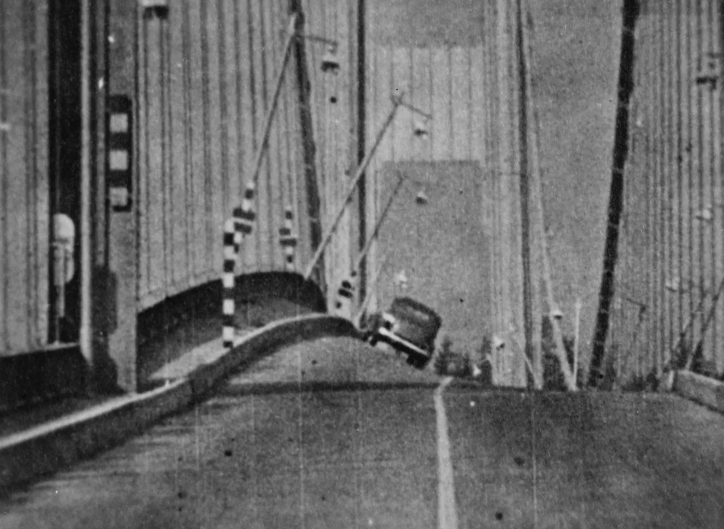
One of the cable bands in mid-span slipped, and the usual vertical rippling was replaced with violent twisting, and both sides of the road sections started falling in opposite directions, as demonstrated in Figure 1 above.4 The twisting grew until hangers fractured and the main span fell into Puget Sound. Investigators were therefore faced with two major questions: why a moderate wind had such a destructive effect as it did and why the bridge could change its mode of movement quickly between vertical and torsional motion.5 The existing scientific knowledge could not easily address these two questions. The flutter theory was created in the 1970s. As a result, quantitative analysis of bridge aerodynamics became feasible. However, the critical wind speeds predicted by Scanlan are significantly different compared to historical and experimental values.6 Scientists have ascribed the difference to increased real damping, differences in the wind and deck angle or lack of certainty in estimating full-scale wind speed. Their explanation matches the observed data that day, both qualitatively and quantitatively, utilizing parametric resonance and Floquet theory.7 It was difficult to do reconstruction because the evidence was thin. The movement was filmed and noted, and the level of full-scale wind speed and damping of the structure at the point of failure could only be estimated, with a gap in how closely theory and observation can be made compatible.8 There was more than one bridge at stake. Any further long-span design must prove to be not a repeat of the failure, and the issue of what model to rely on influenced the way the aerodynamic safety was inspected.
Approach
Recent studies reconstruct the collapse in three complementary ways, including mathematical modeling, wind-tunnel testing and time-domain simulation.
Mathematical Modelling
The research study of Gazzola et al. considered the deck as a nonlinear system and demonstrated how a set of parametric resonances, which can be investigated with Floquet theory, can explain the thresholds witnessed on the day.9 Then, they solve optimal-control and shape-optimization problems with a partial damping term which eliminates energy on the deck to inform the design of future bridges.
Wind-tunnel Testing
Wang et al. conducted an experiment on a 1:25 sectional model of the original deck in a large-amplitude free-vibration rig capable of simulating skew winds.10 They changed wind speed, yaw (0° to 30°), initial attack angle (0° and ±5°) and the structural damping and overlaid torsional aerodynamic damping. A different study employed a full-bridge aeroelastic model (1:110) that recapitulated the large-amplitude anti-symmetric torsional flutter based on a torsional amplitude of 35°.11 The conditions in the test were selected to be similar to the actual bridge. Testing of the sectional tests was in a boundary-layer wind tunnel, Reynolds number 1.99 × 10⁵ with a blockage ratio of 4.6%, in uniform flow and turbulent flow.
Time-domain simulation
The study of Zhang and Zhu drove the experimentally measured, amplitude-dependent aerodynamic forces into a nonlinear finite element model that contains nonlinearity of geometry and materials.12 This approach allowed them to detect the first failing component when the flutter occurred beyond the onset, which is not possible using the classical linear theory of flutter. They compared the model with the actual measured natural frequencies of the bridge; the in-situ first symmetric vertical bending mode measurement was 0.1333 Hz, and the simulation measurement was 0.1329 Hz.
Results
The different research studies covered in the approaches in the preceding section led to a clear picture of the collapse of the bridge, but with a few reservations. First, the torsional flutter could have been the cause of the destructive mechanism. The model of a full bridge replicated torsional flutter of a large amplitude, including alternating symmetric and anti-symmetric flutter.13
The H-shaped deck displays Hopf bifurcation. Depending on the extent of initial disturbance and the speed of the wind, the motion could either vanish or rest on a large limit cycle. When the wind was non-skewed, a subcritical bifurcation was found in some cases, and velocity-restricted flutter in others; a supercritical Hopf bifurcation was the most prevalent pattern which might be useful in explaining the role of having a bridge that might be capable of lasting hours of movement and then shifting behavior at a certain time.14
Hangers, not girders, failed first. At full-bridge with 0° angle of attack, amplitude increased from 20° at 15 m/s to 24° at 18.6 m/s and 32° at 20.4 m/s. At 20.5 m/s the windward quarter-span hanger reached 1,403 MPa, exceeding the 1,250 MPa tensile strength of the cable material, and fractured, with the stiffening girders still in the elastic stage. The order is the same as that of the failure in 1940, and the projections of the simulation were less than 10% off the experimental curves.15
The damping was of great importance in model tests. Added damping reduced torsional amplitude by 30% at a single wind speed and to about 20% of that in the undamped case in a lower range, and turbulent flow generated amplitudes that are half to four-fifths those in uniform flow.16 Neither safeguard was much in the 1940 deck.
Lessons and Takeaways
The dynamic response indicated that the bridge was not safe, while the static wind load indicated it was. Testing of section and full-bridge models in wind tunnels has become common practice, and there is still no other test case for new simulation methods as important as the Tacoma deck. In addition, a streamlined or separated cross-section allows air to flow through or around the device, rather than around the structure to feed vortices. Eight of the 10 longest suspension bridges employ separated/streamlined box girders, and a separated triple-box deck boosted the Messina Straits design flutter critical wind speed to approximately 60 m/s.17 Trade-offs exist with the slots making flutter more stable but increasing vortex-induced vibration, which is why designers use shape and attach other devices like guide vanes. In addition, passive structures like tuned mass dampers and guide vanes, widely studied and adopted, may also be employed, but there is a lack of interest in using them due to their price tag and reliability issues.
However, the hangers themselves became the weak part with the girders remaining elastic. The critical components of the plant can be strengthened, by increasing, for instance, their diameter or quality by a small investment, so that the permissible flutter wind speed is increased. A performance-based approach is proposed in which the vibration amplitude is restricted rather than basing itself on a critical wind speed. Moreover, the direction, damping and nonlinearity of a design are instrumental. Yaw angle, attack angle and damping all affect the flutter behavior, and subcritical bifurcation results in large motion arising from a sufficiently large disturbance even during the subcritical speed. The bridge operated as normal during common wind conditions after opening. The one thing that can be shared is organizational: Motion in a new structure with no explanation, is data. Overall, these lessons provide a foundation for understanding why the modern long span bridges are designed, tested and monitored not just as load carrying structures but also as an aeroelastic system.