
Introduction
I had always been interested in the way buildings appear balanced and visually pleasing even when their parts have different dimensions. I looked at photographs and architectural designs at some point and noted that the width and height of doors, windows, facades and other rectangular features appeared to have selected proportions. The golden rectangles also had the interesting property that removing the square from them left the smaller rectangle with the same proportions. This mathematical property made the Golden Ratio an important topic in geometry and architectural studies. My interest therefore led me to investigate whether the proportions of architectural features was to be modelled using the Golden Ratio. I decided to collect measurements and calculate the ratios independently and not to assume that the building had been designed using φ. This allowed me to compare the actual proportions with the theoretical value of the Golden Ratio.
The investigation was guided by the following research question: To what extent could the proportions of selected architectural features be modelled using the Golden Ratio? I investigated approximately ten rectangular architectural features. For each feature, I measured the longer dimension and shorter dimension and calculated their ratio. I then compared the resulting ratios with . Percentage deviations, the mean, standard deviation and graphical representations were used to determine how closely the architectural measurements followed the theoretical proportion.
Mathematical Background
The Golden Ratio was defined to be the positive solution of the relationship illustrated in the following equation (Atena, 2023, p. 1):
Multiplying both sides by φ gave:
Rearranging produced:
Using the quadratic formula gave:
Therefore:
This value represented the theoretical proportion against which the architectural measurements were compared.
The golden rectangle was the rectangle whose longer side divided by its shorter side was equal to . Therefore, if represented the longer dimension and represented the shorter dimension, the ideal relationship was expressed as shown in the following formula (Akhtaruzzaman et al., 2024, p. 4621).
For the actual architectural measurements, I calculated:
Where represented the observed architectural ratio.
If was close to 1.618, the feature was considered approximately proportional to the golden rectangle.
The percentage deviation from the Golden Ratio was calculated using the following formula:
This provided the standardized way of comparing the different measurements. The smaller percentage deviation represented the closer approximation to the Golden Ratio.
Data Collection
I selected approximately ten rectangular architectural features that were measured consistently. They included larger structural proportions and smaller architectural elements such as entrances, windows and decorative sections. For each feature, I recorded its longer dimension, , and shorter dimension, in the Table 1. The dimensions were then used to calculate the ratio using the formula: .
| Feature | Longer dimension, L (m) | Shorter dimension, S (m) |
|---|---|---|
| 1 | 16.20 | 10.00 |
| 2 | 8.10 | 5.00 |
| 3 | 13.00 | 8.10 |
| 4 | 9.70 | 6.00 |
| 5 | 6.50 | 4.00 |
| 6 | 15.00 | 9.30 |
| 7 | 11.00 | 6.80 |
| 8 | 7.90 | 5.00 |
| 9 | 10.50 | 6.50 |
| 10 | 12.00 | 7.30 |
Calculation of the Architectural Ratio
The architectural ratios were first calculated from the data observed. The sample calculation was carried out for Feature 1.
For Feature 1, the longer dimension was:
and the shorter dimension was:
Therefore:
The architectural ratios of the other features were evaluated using the same method and the results were recorded in the following Table 2.
| Feature | Longer dimension, L (m) | Shorter dimension, S (m) | Architectural Ratio, R |
|---|---|---|---|
| 1 | 16.20 | 10.00 | 1.620 |
| 2 | 8.10 | 5.00 | 1.620 |
| 3 | 13.00 | 8.10 | 1.605 |
| 4 | 9.70 | 6.00 | 1.617 |
| 5 | 6.50 | 4.00 | 1.625 |
| 6 | 15.00 | 9.30 | 1.613 |
| 7 | 11.00 | 6.80 | 1.618 |
| 8 | 7.90 | 5.00 | 1.580 |
| 9 | 10.50 | 6.50 | 1.615 |
| 10 | 12.00 | 7.30 | 1.644 |
The calculated architectural ratios were used to plot the graph to determine the way the calculated ratios were distributed using the Excel software as illustrated in the following Figure 1.
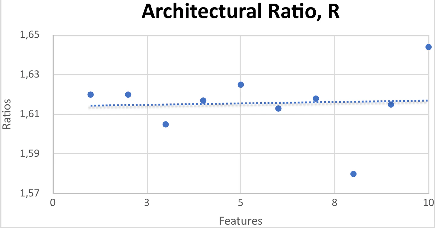
The Figure 1 showed that the calculated ratios varied between 1.580 and 1.644. This variation was important because it allowed me to determine whether the Golden Ratio described most of the architectural features or only a small number of them.
Calculation of the Percentage Deviation of the Architectural Ratio from the Golden Ratio
The theoretical Golden Ratio was:
Therefore, the difference between the observed ratio and the theoretical ratio was first evaluated using the following equation:
The percentage deviation was then calculated as follows:
This indicated that Feature 1 had a very small deviation from the Golden Ratio.
For comparison, Feature 8 had:
Therefore:
Its percentage deviation was:
Feature 8 therefore deviated more substantially from the theoretical Golden Ratio than Feature 1. Therefore, the percentage deviations for the other features were evaluated using the same formula and recorded in the Table 3 for better comparison.
| Feature | Observed ratio | Golden Ratio | Percentage deviation |
|---|---|---|---|
| 1 | 1.620 | 1.618 | 0.12% |
| 2 | 1.620 | 1.618 | 0.12% |
| 3 | 1.605 | 1.618 | 0.80% |
| 4 | 1.617 | 1.618 | 0.06% |
| 5 | 1.625 | 1.618 | 0.43% |
| 6 | 1.613 | 1.618 | 0.31% |
| 7 | 1.618 | 1.618 | 0.00% |
| 8 | 1.580 | 1.618 | 2.35% |
| 9 | 1.615 | 1.618 | 0.19% |
| 10 | 1.644 | 1.618 | 1.61% |
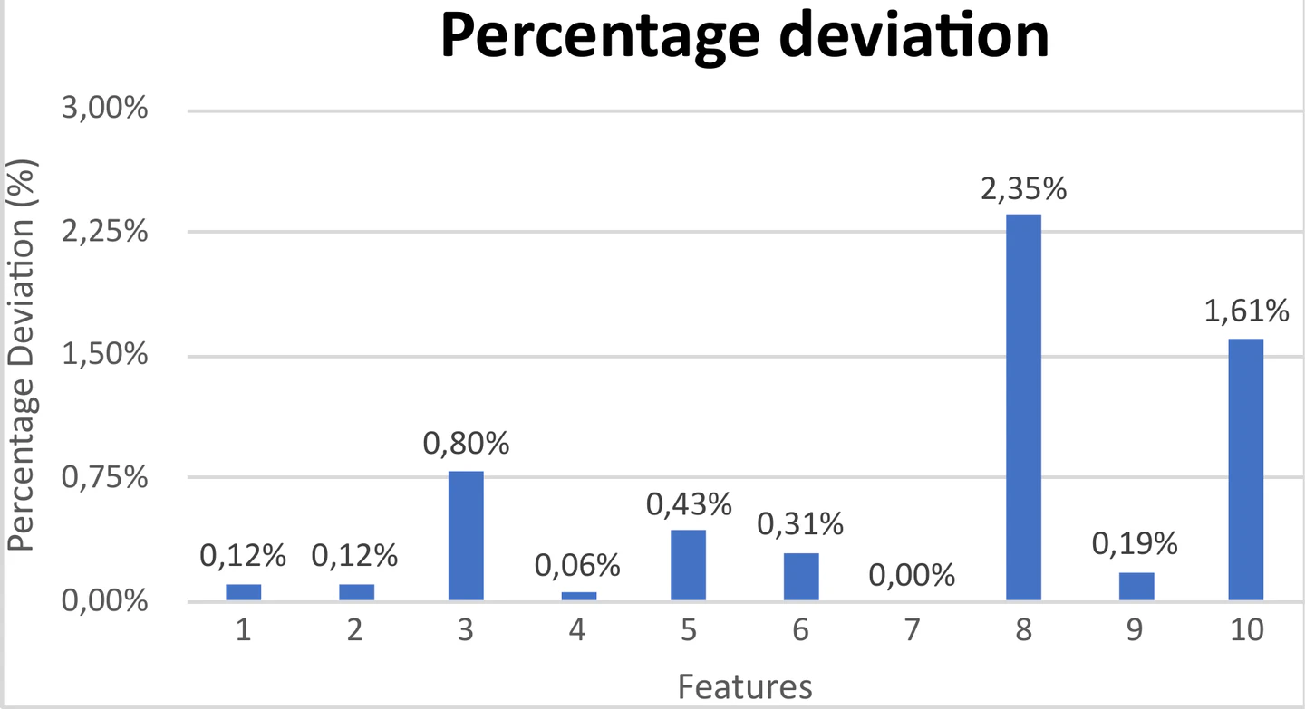
The results in the Figure 2 showed that most of the features had relatively small deviations. Feature 7 produced the observed ratio of 1.618, which was equal to the theoretical value at the precision used. Feature 4 had the smallest non-zero deviation of 0.06%. Feature 8 had the largest deviation 2.35% and this indicated that although the Golden Ratio appeared to provide the reasonable model for many of the selected features, it did not describe every feature equally well.
Mean Architectural Ratio
To determine the overall relationship between the measurements and the Golden Ratio, I calculated the arithmetic mean.
The mean was calculated using:
Where:
Using the ten calculated ratios:
Rounded to three decimal places:
The theoretical Golden Ratio was:
The difference was:
The absolute difference was:
The percentage deviation of the mean was therefore:
The percentage deviation of approximately 0.12% was small and indicated that the average architectural proportion was very close to the Golden Ratio. However, the mean alone could have hidden differences between individual measurements. Therefore, I calculated the standard deviation.
Standard Deviation
Although the mean ratio indicated how closely the architectural proportions followed the Golden Ratio, it did not show how much the individual ratios varied around the mean. I therefore calculated the sample standard deviation.
The ten observed ratios were:
1.620, 1.620, 1.605, 1.617, 1.625, 1.613, 1.618, 1.580, 1.615, 1.644
The mean used in the calculation was:
The sample standard deviation was calculated using:
Where:
Since there were ten measurements:
Therefore:
Step 1: Calculate the deviations from the mean
For Feature 1:
For Feature 2:
For Feature 3:
The same process was repeated for all ten measurements.
| Feature | Ratio, | ||
|---|---|---|---|
| 1 | 1.620 | 0.004 | 0.000016 |
| 2 | 1.620 | 0.004 | 0.000016 |
| 3 | 1.605 | −0.011 | 0.000121 |
| 4 | 1.617 | 0.001 | 0.000001 |
| 5 | 1.625 | 0.009 | 0.000081 |
| 6 | 1.613 | −0.003 | 0.000009 |
| 7 | 1.618 | 0.002 | 0.000004 |
| 8 | 1.580 | −0.036 | 0.001296 |
| 9 | 1.615 | −0.001 | 0.000001 |
| 10 | 1.644 | 0.028 | 0.000784 |
| Total | 0.002329 |
Therefore:
Substituting into the standard-deviation formula:
Therefore, to three decimal places:
The standard deviation of approximately 0.016 indicated that the architectural ratios were relatively closely distributed around the mean value of 1.616. Feature 8 and Feature 10 were further from the mean than most of the other observations and therefore contributed more substantially to the variation.
Interpretation of the Mathematical Results
The mathematical analysis was used to determine how closely the selected architectural proportions corresponded to the Golden Ratio. The theoretical value was 1.6180 and the ten architectural features produced ratios ranging from 1.580 to 1.644. The calculated mean was 1.616 and the difference between the mean and the theoretical Golden Ratio was 0.002. The percentage deviation was 0.12% and it indicated that the average architectural proportion was very close to the Golden Ratio. The result therefore suggested that provided a reasonable mathematical model for the overall proportions of the selected features. The mean did not provide enough information about the variation between individual features. The standard deviation was approximately 0.016 and it showed that the observed ratios were generally concentrated around the mean of 1.616. Features 1 and 2 both had ratios of 1.620, while Feature 7 had a ratio of 1.618. Feature 4 also produced a ratio of 1.617. These values were very close to the theoretical Golden Ratio. In contrast, the Feature 8 had a ratio of 1.580 and Feature 10 had a ratio of 1.644. These features were further from the theoretical value and contributed more to the overall variation. The percentage deviation analysis provided further evidence. Eight of the ten features had percentage deviations below 1%. Feature 7 had almost no deviation, while Feature 8 had the greatest deviation at approximately 2.35%. Therefore, the results showed that the Golden Ratio provided a close approximation for most of the selected architectural features, although it did not describe every feature exactly.
Evaluation of the Mathematical Model
The investigation had several strengths. One important strength was that I converted an initial visual observation into a quantitative mathematical investigation. Rather than deciding that the architecture appeared to contain the Golden Ratio based only on appearance, I measured dimensions, calculated ratios and compared them with the theoretical value of φ. The second strength was the use of multiple architectural features. Measuring ten features provided more evidence than relying on a single ratio. This allowed me to determine whether the apparent relationship with the Golden Ratio occurred across several parts of the architecture. The use of several mathematical techniques also strengthened the investigation. The ratio provided the fundamental measurement. Percentage deviation showed how close each feature was to . The mean provided the overall measure of the architectural proportions, while the standard deviation showed how much the individual ratios varied around the mean. Figure 1 allowed the observed ratios to be compared visually with the theoretical Golden Ratio, while Figure 2 showed the relationship between the individual observations and 1.618. Another strength was that the investigation did not assume that every architectural measurement had to equal exactly 1.618. This made the mathematical model more realistic because physical measurements were unlikely to correspond perfectly to an irrational number.
Limitations
Despite the strengths, several limitations varied the reliability of the investigation. The first limitation concerned measurement accuracy. The architectural dimensions were obtained scaled images and perspective distortion varied the apparent dimensions. The features were selected because their dimensions could be identified and measured. This could have introduced selection bias because some architectural elements may have been excluded due to difficulties in measuring them. Another limitation was that the investigation focused on rectangular or approximately rectangular proportions. Other architectural features, such as arches, domes, circular designs and irregular geometric patterns, were not represented by the simple ratio .
Improvements to the Investigation
Several improvements could have increased the reliability and mathematical depth of the investigation. First, I could have increased the sample size by measuring at least 30 architectural features. Second, I could have used the systematic sampling method. Instead of selecting features based on convenience, I could have identified all measurable rectangular features and assigned each one a number. A random selection procedure could then have been used to choose the features for analysis. This would have reduced selection bias. Third, the accuracy of the measurements could have been improved by using architectural plans, technical drawings as well as orthographic projections rather than photographs. This would have reduced errors caused by perspective and image distortion.
Reflection on the Investigation
At the beginning of the investigation, I was interested in whether the balanced appearance of architectural structures could be explained by a mathematical relationship. I initially expected that several of the selected proportions might be close to the Golden Ratio because of the apparent visual balance of the architecture. The mathematical analysis provided a more detailed result. The total average of 1.616 was close to 1.618 and it supported my initial observation that there might be a relationship between architectural proportions and the Golden Ratio.
Conclusion
The investigation was guided by the research question: To what extent could the proportions of selected architectural features be modelled using the Golden Ratio? The theoretical Golden Ratio that was used was 1.618 and the observed ratios ranged from 1.580 to 1.644, while the calculated mean was 1.616. The difference between the mean and the theoretical Golden Ratio was 0.002 and it produced the percentage deviation of approximately 0.12%. The sample standard deviation, using the requested mean of 1.616, was approximately 0.016 and it indicated that the ratios were relatively closely grouped around the mean. Eight of the ten architectural features had percentage deviations below 1%, showing that most of the selected proportions were reasonably close to the Golden Ratio. The results therefore indicated that the Golden Ratio provided a close mathematical model for the overall proportions of the selected architectural features. The mean was particularly close to 1.618, and the majority of the individual measurements supported this relationship. Therefore, the answer to the research question was that the selected architectural proportions could be modelled closely using the Golden Ratio at an overall level, but the Golden Ratio did not describe every individual feature exactly.