Pendulum Length and Period: IB Physics IA

This IB Physics Internal Assessment asks how the length of a simple pendulum, from 0.20 m to 1.00 m, affects its period of oscillation when the initial angle is kept at 20°. The data come from the PhET Pendulum Lab simulation, not from a pendulum set up in a laboratory: five timed trials at each length, with the mass, gravity and friction fixed on screen. The mean periods are processed with their uncertainties into graphs of the period squared against length and of ln T against ln L, which give an exponent of 0.500 ± 0.019 and g = 9.81 ± 0.25 m s⁻² once the 20° amplitude correction is applied.

Research Question

How does the length of a simple pendulum (0.20, 0.40, 0.60, 0.80 and 1.00 ± 0.01 m) affect its period of oscillation while keeping the initial angular displacement constant at 20°?

Introduction

The simple pendulum provides an easily constructed device for the investigation of the relationship between oscillatory motion and the physical factors which affect it. The factors influencing the motion of a pendulum include the length of the pendulum, period, mass, and angle of inclination, concepts learned in IB Physics. However, I have been interested in understanding the exact relationship between the length and the period of the pendulum. Thus, this investigation was chosen to gain further insight into simple harmonic motion and would allow me to answer the question set: What will the effect on the time taken to complete one oscillation be when the length of the pendulum is varied. The importance of this investigation lies in its use of the pendulum motion to demonstrate how a physical system can be modeled using mathematics, and how a relationship between two physical variables can be tested using experiment. The knowledge of how things influence a pendulum's period of oscillation will also help your comprehension of aspects of historic timepieces and experimental procedures which are used to estimate the magnitude of gravitational acceleration. In addition, calculation of deviation from values predicted by theory and uncertainties in the measurements will show the limits of validity of idealized models, particularly at small angles.

Theoretical Background

A simple pendulum is composed of a point mass (the bob) that is attached to an inextensible string, as displayed in Figure 1 below. The string of the pendulum bob is of a length $L$ , and the entire pendulum is displaced through an angle $θ$ . In its operation, the pendulum contains a mass oscillating at the end of the pendulum, swinging back and forth due to gravity's pull.

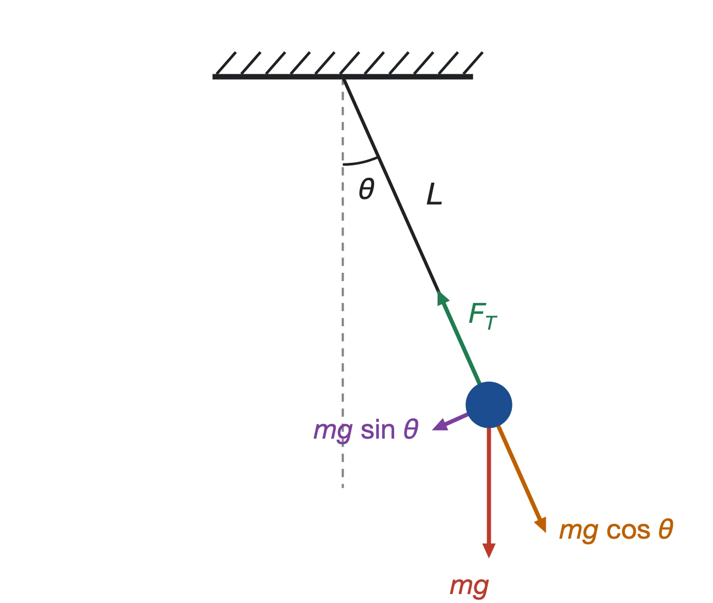
Diagram of a simple pendulum: a bob hangs from a fixed support on a string of length L, displaced by an angle θ from the dashed vertical. Arrows on the bob show the tension F_T along the string towards the support, the weight mg straight down, its component mg cos θ along the string away from the support and its component mg sin θ at right angles to the string, back towards the vertical. — Figure 1: The Set-up of the Simple Pendulum Bob (adapted from Elert, 2025)

When the above pendulum is displaced through the angle $θ$ , the net restoring force acting on it is expressed through the equation:

F = - m g \sin θ

For small angles, $\sin θ \approx θ$

The acceleration is then proportional and opposite to the displacement, which is simple harmonic motion with angular frequency $ω = \sqrt{g / L}$ . Hence

Period, T = 2 π \sqrt{\frac{L}{g}}

\Rightarrow T^{2} = \frac{4 π^{2}}{g} L

The mass cancels. Thus, the period depends only on $L$ and $g$ . A graph of $T^{2}$ against $L$ should be linear through the origin with gradient $4 π^{2} / g$ , which allows $g$ to be determined.

The small-angle approximation is not exact at 20°. For an amplitude $θ_{0}$ (in radians) the period is

T = T_{0} (1 + \frac{θ_{0}^{2}}{16} + \frac{11 θ_{0}^{4}}{3072} + \dots)

Where:

T_{0} = 2 π \sqrt{L / g}

For $θ_{0} = 20° = 0.349 rad$ , the bracket is 1.0077. Thus, the period can be predicted to be 0.77 % longer than $T_{0}$ at every length. This factor is independent of $L$ , so $T \propto L^{0.5}$ still holds, but the gradient of $T^{2}$ against $L$ rises from 4.024 to 4.086 s² m⁻¹.

A power law $T = k L^{n}$ becomes linear after taking natural logarithms, according to the past research study of Roman and Bertolotti (2022):

\ln T = \ln k + n \ln L

Thus, the gradient of $\ln T$ against $\ln L$ gives the exponent $n$ directly, without needing $g$ .

In conducting this investigation for the determination of how the length of a simple pendulum affects its period of oscillation while keeping the initial angular displacement constant at 20°, an online PhET Interactive Simulations (2026) simulation would be used, as it allows fixing of both the mass and gravitational acceleration and also reduces friction by eliminating air resistance and human reaction time.

Hypothesis

It is hypothesized that an increase in the magnitude of the length of the pendulum will lead to a corresponding increase in its period. Thus:

T² against L will be linear through the origin with a gradient of about 4.09 s² m⁻¹ (g = 9.81 m s⁻², including the 20° correction);
ln T against ln L will be linear with a gradient of 0.5.

This hypothesis is based on the theoretical equation:

T = 2 π \sqrt{L / g}

A longer string gives a longer arc and a smaller restoring acceleration $g / L$ for the same angle. Mass is not expected to affect the period.

Variables

Table 1: The Main Variables, Operational Definitions and Measurement/Variation
Variable	Definition of Variable	Variation/Measurement
Independent	Pendulum length, L	Set to 0.20, 0.40, 0.60, 0.80 and 1.00 m using the length control (± 0.01 m)
Dependent	Period of oscillation, T	Read from the Period Timer over 10 oscillations (± 0.0001 s)

Table 2: Control Variables and Mechanism Adopted for Control
Controlled variable	How it is controlled	Why it is controlled
Initial angle	The bob was dragged to the twenty-degree mark of the on-screen protractor and released from rest every time.	The period increases slightly with amplitude so that a different starting angle would change the period.
Mass of bob	Fixed at one kilogram.	Ensures that any change in the period is due to the length only.
Gravitational field	The "Earth" setting would be used throughout the experiment.	The period depends on the gravitational field strength, so it must not change.
Friction	Slider kept at "None".	Damping would reduce the amplitude and alter the period.
Timing method	The Period Timer was used for all trials, over ten oscillations.	Removes reaction-time error and treats every length identically.

Materials and Equipment

Table 3: The Main Materials and Equipment Used in the Experiment
Equipment/Material	Quantity and Specification
Computer with internet browser	1
PhET Pendulum Lab simulation	1, latest HTML5 version (PhET Interactive Simulations, 2026)
On-screen protractor	Used to set 20°
On-screen length control and ruler	Resolution ± 0.01 m
On-screen Period Timer	Resolution ± 0.0001 s

Pilot Experiment

Pilot trials at 0.80 m were used to check that the bob could be released reliably from 20°, that the Period Timer readings repeated to within the fourth decimal place, and that the period stayed steady over ten oscillations with friction on "None". Since the readings agreed so closely, five trials per length were judged sufficient.

Procedure

The online simulation was first opened and the ruler and protractor placed at their positions.
The mass of the pendulum was then set to 1.00 kg, and gravity set to Earth (9.81 m s⁻²).
The length of the string was then set to the first treatment value of 0.20 m.
The pendulum bob was then dragged in the simulation to an angle of 20° mark using a protractor.
The Period Timer was started and the bob was released from rest. The period was recorded after 10 oscillations, to four decimal places.
The pendulum was reset and steps 3–5 were repeated until five trials had been recorded.
Steps 2–6 were repeated for lengths of 0.40, 0.60, 0.80 and 1.00 m.

Risk Assessment

Table 4: Safety, Ethical and Environmental Considerations
Hazard	Risk	Control Measures
Prolonged screen use	Eye strain and poor posture	Sat correctly, with a short break every 20 minutes
Laptop charger and cables	Tripping and electric shock	Cables kept out of walkways and dry

Since the experiment did not involve the use of animals and plants, there were no major ethical considerations that were to be made. The only major ethical consideration was the computer's energy use, which was controlled by opening the computer only while conducting the experiment.

Raw Data

The raw data on the measured periods of the pendulum system measured in the experiment in all the variations of the length were recorded into Table 5 below. These data would be utilized in data processing for effective determination of the effect of varying length on the measured period of the pendulum at a fixed angle of 20°.

Table 5: Period of the Pendulum, T (± 0.0001 s), for Five Trials at Each Length
Length, $L$ (± 0.01 m)	Trial 1	Trial 2	Trial 3	Trial 4	Trial 5
0.20	0.9040	0.9042	0.9040	0.9043	0.9040
0.40	1.2785	1.2785	1.2784	1.2788	1.2784
0.60	1.5658	1.5655	1.5659	1.5656	1.5658
0.80	1.8080	1.8083	1.8080	1.8082	1.8083
1.00	2.0215	2.0214	2.0217	2.0215	2.0214

Sample Calculations and Data Processing

Sample Calculations of Period and Uncertainties

For each length the mean period and its uncertainty were first calculated using the following general formulas:

Mean Period of the simple pendulum, \overline{T} = \frac{T_{Trial 1} + T_{Trial 2} + T_{Trial 3} + T_{Trial 4} + T_{Trial 5}}{5}

Uncertainty of Period, Δ \overline{T} = \frac{T_{max} - T_{min}}{2}

Sample calculations were conducted using the values corresponding to the length of 0.60 m, from Table 5 above:

Mean Period of the simple pendulum, \overline{T} = \frac{1.5658 + 1.5655 + 1.5659 + 1.5656 + 1.5658}{5} = 1.56572 s

Uncertainty of Period, Δ \overline{T} = \frac{1.5659 - 1.5655}{2} = 0.0002 s

This value is larger than the timer resolution (0.0001 s), so it was used as the uncertainty in $\overline{T}$ . These calculations were extended to all the variations of lengths and the results obtained recorded into the processed data Table 6 below.

The calculated values were then used to compute $T^{2}$ , $\ln L$ and $\ln T$ with propagated uncertainties. The 0.60 m data are used as the sample.

\overline{T} = \frac{1.5658 + 1.5655 + 1.5659 + 1.5656 + 1.5658}{5} = 1.56572 s

Δ \overline{T} = \frac{T_{max} - T_{min}}{2} = \frac{1.5659 - 1.5655}{2} = 0.0002 s

Squaring the mean period, the uncertainty is doubled in fractional terms:

{\overline{T}}^{2} = {1.56572}^{2} = 2.4515 s^{2}

Δ ({\overline{T}}^{2}) = 2 \overline{T} Δ \overline{T} = 2 (1.56572) (0.0002) = 0.0006 s^{2}

For the logarithms:

\ln L = \ln 0.60 = - 0.511

Δ (\ln L) = \frac{Δ L}{L} = \frac{0.01}{0.60} = 0.017

\ln \overline{T} = \ln 1.56572 = 0.4483

Δ (\ln \overline{T}) = \frac{Δ \overline{T}}{\overline{T}} = \frac{0.0002}{1.56572} = 0.0001

The theoretical period at 20° is:

T = 2 π \sqrt{\frac{0.60}{9.81}} \times 1.0077 = 1.5658 s

The theoretical value matches with the $\overline{T}$ .

The same calculations were applied to every length. The results are in Table 6.

Table 6: Processed Data for the Mean Period, T̄² and Natural Logarithms with their Uncertainties
$L$ (m)	$\overline{T} \pm Δ \overline{T}$ (s)	${\overline{T}}^{2} \pm Δ$ (s²)	$\ln (L / m) \pm Δ$	$\ln (\overline{T} / s) \pm Δ$
0.20	0.9041 ± 0.0002	0.8174 ± 0.0003	−1.609 ± 0.050	−0.1008 ± 0.0002
0.40	1.2785 ± 0.0002	1.6346 ± 0.0005	−0.916 ± 0.025	0.2457 ± 0.0002
0.60	1.5657 ± 0.0002	2.4515 ± 0.0006	−0.511 ± 0.017	0.4483 ± 0.0001
0.80	1.8082 ± 0.0002	3.2694 ± 0.0005	−0.223 ± 0.013	0.5923 ± 0.0001
1.00	2.0215 ± 0.0002	4.0865 ± 0.0006	0.000 ± 0.010	0.7038 ± 0.0001

Graphical Plots and Analysis

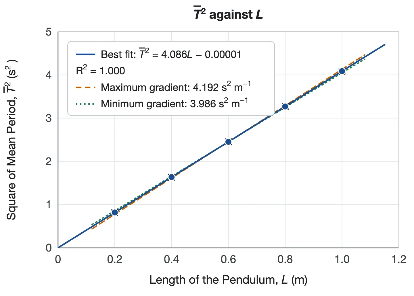
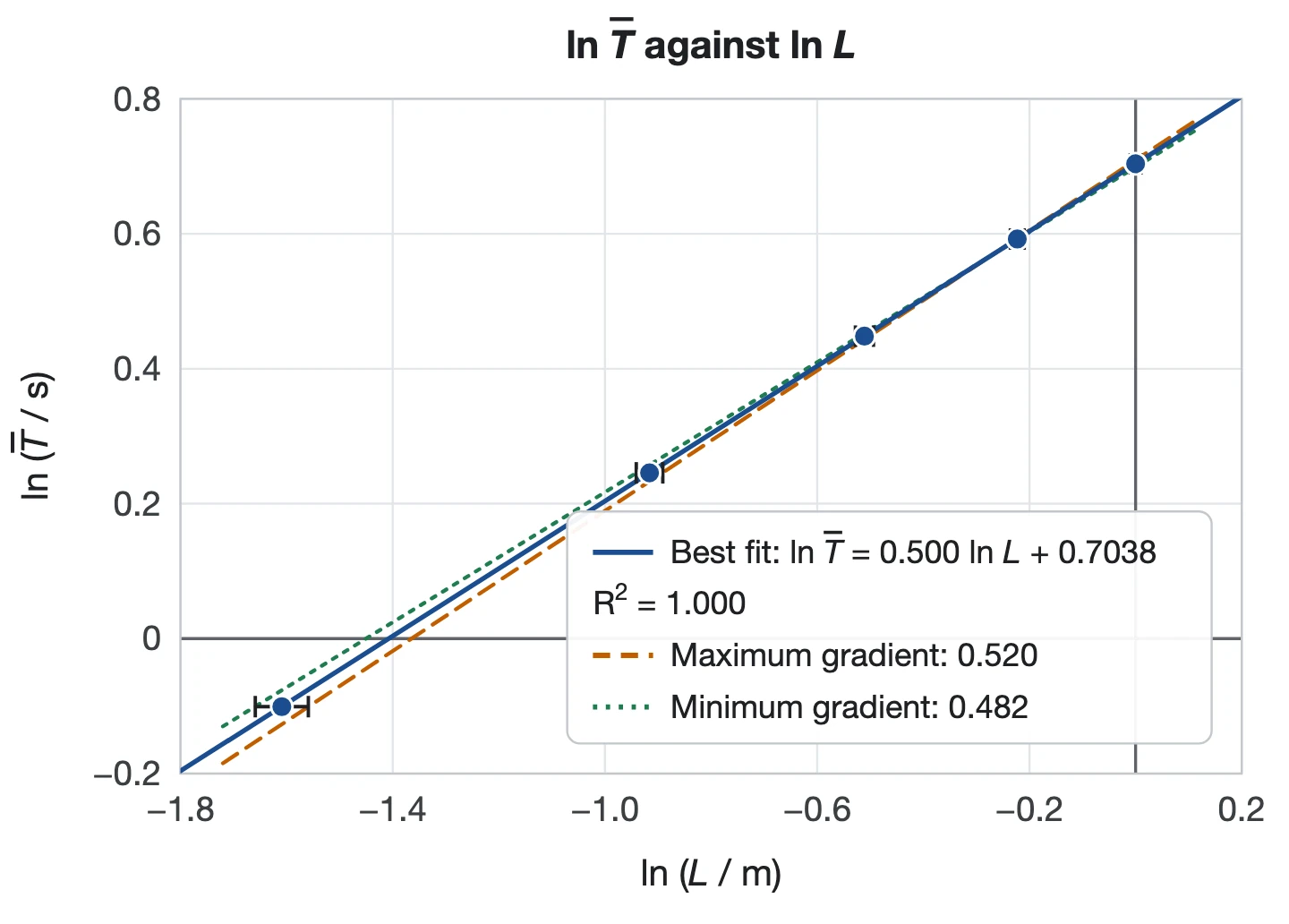
The data were plotted with error bars, a least-squares best-fit line, and maximum and minimum gradient lines drawn through the extremes of the error bars. The graph was plotted using the MS Excel.

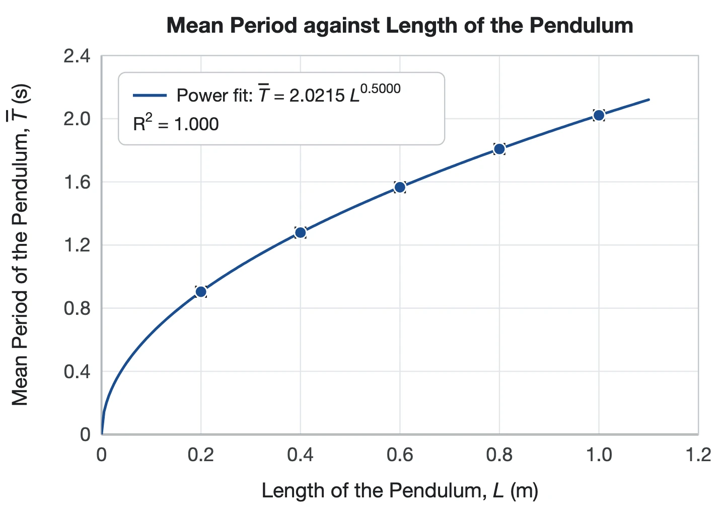
Graph of the mean period T̄ in seconds against the pendulum length L from 0 to 1.2 m. The five points, 0.9041 s at 0.20 m, 1.2785 s at 0.40 m, 1.5657 s at 0.60 m, 1.8082 s at 0.80 m and 2.0215 s at 1.00 m, lie on a rising curve that flattens as the length grows: the power fit T̄ = 2.0215 L^0.5000 with R² = 1.000. — Figure 2: A Graph of Mean Period against Length of the Pendulum

The relationship between the mean period and the length of the pendulum is in the power law:

T = k L^{n}

T = 2.0215 L^{0.5}

Graph of the square of the mean period, T̄² in s², against the length L in m. The five points, from 0.8174 s² at 0.20 m to 4.0865 s² at 1.00 m, lie on a straight line through the origin: best fit T̄² = 4.086L − 0.00001 with R² = 1.000. A dashed maximum-gradient line (4.192 s² m⁻¹) and a dotted minimum-gradient line (3.986 s² m⁻¹) pass through the ends of the error bars of the first and last points. — Figure 3: Graph of T² against L

Graph of ln T̄ against ln L. The five points, from (−1.609, −0.1008) to (0.000, 0.7038), with horizontal error bars from ± 0.050 at the shortest length to ± 0.010 at the longest, lie on a straight line: best fit ln T̄ = 0.500 ln L + 0.7038 with R² = 1.000. A dashed maximum-gradient line (0.520) and a dotted minimum-gradient line (0.482) pass through the ends of the error bars of the first and last points. — Figure 4: A Graph of Ln T against Ln L

The slopes of all the curves plotted in this investigation were as displayed in Table 7 below.

Table 7: Best-Fit and Slopes
Graph	Best-fit gradient	Uncertainty, $Δ s$
T̄² vs L	4.086 s² m⁻¹	± 0.103
ln T̄ vs ln L	0.500	± 0.019

The graph presented in Figure 2 above shows that the period rises with length with a decreasing slope, so the relationship is not linear. In Figure 3, ${\overline{T}}^{2}$ is directly proportional to $L$ : the gradient is 4.086 ± 0.103 s² m⁻¹, the intercept is −0.00001 s² (zero within uncertainty) and the correlation coefficient is 1.000. The experimental gravitational field strength is

g = \frac{4 π^{2}}{gradient} = \frac{4 π^{2}}{4.086} = 9.66 \pm 0.24 m s^{- 2}

This value is 1.5 % below 9.81 m s⁻², but within the uncertainty. Dividing the gradient by the amplitude factor 1.0077² = 1.0154 gives $g = 9.81 \pm 0.25 m s^{- 2}$ , in agreement with the set value, showing that the 20° correction matters.

In Figure 4 the gradient is $n = 0.500 \pm 0.019$ , which agrees with the predicted 0.5. The intercept $\ln k = 0.7038$ gives $k = 2.0215 s m^{- 0.5}$ , against a theoretical $2 π / \sqrt{9.81} \times 1.0077 = 2.0215 s m^{- 0.5}$ . Every measured period also lies within 0.01 % of the 20° theoretical value but 0.76–0.78 % above the small-angle value $T_{0}$ .

Conclusion

The aim of this investigation was to determine how the length of a simple pendulum affects its period of oscillation while keeping the initial angular displacement constant at 20°. In conducting the investigation, it had been hypothesized that increase in the magnitude of the length of the pendulum would lead to a corresponding increase in its period. The period increased from 0.9041 s to 2.0215 s as length increased fivefold, with an exponent of $n = 0.500 \pm 0.019$ in agreement with 0.5, and ${\overline{T}}^{2}$ was directly proportional to $L$ with a zero intercept. The hypothesis was therefore supported. The gradient of ${\overline{T}}^{2}$ against $L$ gave $g = 9.66 \pm 0.24 m s^{- 2}$ , and $9.81 \pm 0.25 m s^{- 2}$ once the 20° amplitude correction was applied, matching the simulation’s value. Hence, the hypothesis was supported. The data also confirm that the small-angle formula underestimates the period by about 0.77 % at 20°.

Evaluation

Table 8: Limitations, their Effects and Improvements
Limitation	Effect on results	Improvement
Length uncertainty of ± 0.01 m is 5 % of the 0.20 m length	It dominates the gradient uncertainties, since the spread in T is only about 0.0002 s.	Use the ruler to confirm each length precisely and use longer lengths where the relative uncertainty is smaller.
Only five lengths between 0.20 m and 1.00 m	ln L spans a narrow range, the fits had few points and the intercept is less certain.	Use ten lengths from 0.10 m to 1.00 m.
Only one amplitude (20°)	The θ₀²/16 correction was compared only indirectly with theory.	Repeat at several amplitudes (5°–60°) and compare T with theory.
Idealized simulation	No friction, air resistance or string mass, so periods are nearly identical and ΔT underestimates real variation.	Repeat with a real pendulum and a light gate to compare the results.
Average of 10 oscillations	Individual-period variation is hidden.	Record several single periods.

Physics IA: Pendulum Length and Period

Research Question

Introduction

Theoretical Background

Hypothesis

Variables

Materials and Equipment

Pilot Experiment

Procedure

Risk Assessment

Raw Data

Sample Calculations and Data Processing

Sample Calculations of Period and Uncertainties

Graphical Plots and Analysis

Conclusion

Evaluation

References

Rate This Sample

Cite This Sample

We'll ensure your essay is what you asked for

Research Question

Introduction

Theoretical Background

Hypothesis

Variables

Materials and Equipment

Pilot Experiment

Procedure

Risk Assessment

Raw Data

Sample Calculations and Data Processing

Sample Calculations of Period and Uncertainties

Graphical Plots and Analysis

Conclusion

Evaluation

References

Rate This Sample

Cite This Sample

Calculating the Volume of a Vase

Correlation between HIV mortality and GDP

Dice Probability and Expected Rent in Monopoly